Modeling Influence with Graphs

Graphs, $G = (V, E) $	$N \times N $ Adjacency Matrix	$N \times L $ Incidence Matrix
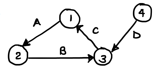	$A = \begin{bmatrix}0 & 1 & 0 & 0 \\ 0 & 0 & 1 & 0 \\ 1 & 0 & 0 & 0 \\ 0 & 0 & 0 & 1\end{bmatrix} $	$\hat{A} = \begin{bmatrix}1 & 0 & -1 & 0 \\ -1 & 1 & 0 & 0 \\ 0 & -1 & 1 & -1 \\ 0 & 0 & 0 & 1\end{bmatrix} $
$ V $ = set of $ N $ nodes $ E $ = set of $ L $ links	$ A_{ij} = 1 $ iff $ (i, j) \in E $ Note that $A$ need not be symmetric for directed graphs.	For a directed graph, $ A_{ij} $ is $1$ if $ i $ starts at $ j $; $-1$ if $i$ ends at $j$, and $0$ otherwise. For an undirected graph, $A_{ij}$ is $1$ if $i$ on $j$, and $0$ otherwise.

Measurements of Node Importance

For undirected graphs, this is the number of nodes connecting to node $i$.

For directed graphs, we have a separate in-degree and out-degree centralities.

$\vec{x}$ is the solution to $ A\vec{x} = \lambda_1 \vec{x} $, i.e. the eigenvector corresponding to $ \lambda_1 $, the largest eigenvalue for $A$.

We pick $ \lambda_1 $ because in the power series $ \vec{x}[t] = A^t \vec{x}[0] $, the largest $\lambda$ of $A$ will dominate as $t \to \infty $.

This means that $ x_i = \frac{1}{\lambda_1} \sum_{j} A_{ij} x_j\ \ \forall i $, and that we can also normalize $ \vec{x}$.

Let $ d_{ij} $ be the shortest path distance from $i$ to $j$.

$$ C_i = \frac{n-1}{\sum_{j \ne i} d_{ij}} $$

$ C_i $ is the reciprocal of the average shortest distance from $i$ to the other nodes.

Tip: the largest $d_{ij}$ across all $(i,j)$ is the diameter of the network.

Let $ n_{st}^{i} $ be the number of shortest paths for pair $(s, t)$ that $i$ sits on.

Let $ g_{st} $ be the total number of shortest paths between nodes $s$ and $t$.

$$ B_i = \sum_{s \ne i} \sum_{t < s} \frac{n_{st}^{i}}{g_{st}} $$

Between centrality assumes that important nodes are on the shortest paths of many other pairs.

Closeness and betweeness may be inconsistent, e.g. small world graphs have uniform closeness, but varying betweeness.

The Medicis had $ \times 1.5 $ degree, but $ \times 5 $ betweeness centrality.

$$ B_{(i, j)} = \sum_{s} \sum_{t < s} \frac{ n_{st}^{(i, j)} }{ g_{st}} $$

Links can be defined differently, e.g. friends, friends that chat, followers, etc.

An important link has a strong weight, or might glue the network together.

Locally important links connect few specific nodes with no common neighbors. Globally important links connect many node pairs.

A weak link connects nodes that otherwise have little overlap. These are important precisely for opening up communication channels.

Graphs, \(G = (V, E) \)	\(N \times N \) Adjacency Matrix	\(N \times L \) Incidence Matrix
	\(A = \begin{bmatrix}0 & 1 & 0 & 0 \\ 0 & 0 & 1 & 0 \\ 1 & 0 & 0 & 0 \\ 0 & 0 & 0 & 1\end{bmatrix} \)	\(\hat{A} = \begin{bmatrix}1 & 0 & -1 & 0 \\ -1 & 1 & 0 & 0 \\ 0 & -1 & 1 & -1 \\ 0 & 0 & 0 & 1\end{bmatrix} \)
\( V \) = set of \( N \) nodes \( E \) = set of \( L \) links	\( A_{ij} = 1 \) iff \( (i, j) \in E \) Note that \(A\) need not be symmetric for directed graphs.	For a directed graph, \( A_{ij} \) is \(1\) if \( i \) starts at \( j \); \(-1\) if \(i\) ends at \(j\), and \(0\) otherwise. For an undirected graph, \(A_{ij}\) is \(1\) if \(i\) on \(j\), and \(0\) otherwise.