Note: similarity indexes may not specify the 4 NIST specifications of a similarity metric .
Russel-Rao
Where \(|q|\) is the total number of binary features considered:
$$ f(q, d) = \frac{ CP(q, d) + CA(q, d) }{ |q| } $$
This similarity measure is used by Netflix.
Sokal-Michener
$$ f(q, d) = \frac{ CP(q, d) + CA(q, d) }{ |q| } $$
This is useful for medical diagnoses.
Jaccard Index
$$ f(q, d) = \frac{ CP(q, d) }{ CP(q, d) + PA(q, d) + AP(q, d) } $$
e.g. for a retailer, the list of customer-items are sparse. Co-absences are not important.
It’s probably more than that. Co-absences would dominate the predictions despite having little value.
Cosine Similarity
$$ f(q, d) = \frac{ \sum_{i=1}^{m} (q_i \cdot d_i) }{ \sqrt{ \sum_{i=1}^{m} q_i^2 } \times \sqrt{ \sum_{i=1}^{m} d_i^2 } } = \frac{\vec{q} \cdot \vec{d}}{ |\vec{q}| \times |\vec{b}| } $$
The result ranges from \(0\) (dissimilar) to \(1\) (similar).
The measure only cares about the angle between the two vectors. The magnitudes of the vectors are inconsequential.
Sanity check: say we have \(q = (7, 7)\) and \(d = (2, 2)\):
$$ f(q, d) = \frac{ 7 \cdot 2 + 7 \cdot 2 }{ \sqrt{7^2 + 7^2} \times \sqrt{ 2^2 + 2^2 }} = 1 $$
Looks like cosine similarity is a trend-finder. I’m uncomfortable that \((2, 2)\) is considered to be as close to \( (1, 1)\) as it is to \( (7, 7) \).
Mahalanobis Distance
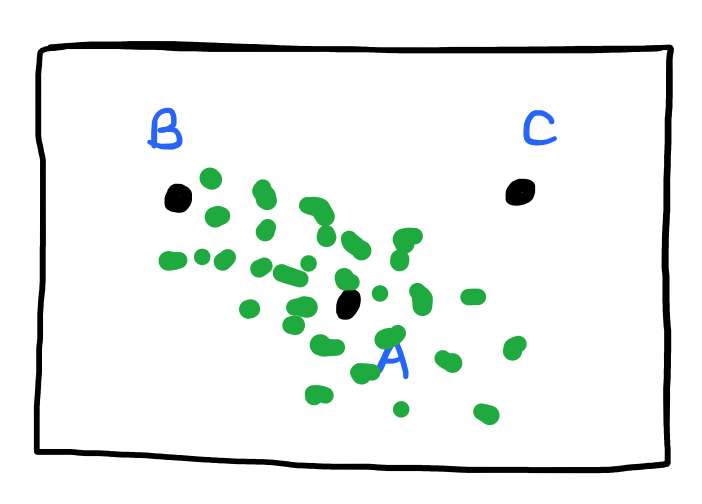
$$ f\left(\vec{a}, \vec{b}\right) = \begin{bmatrix} a_1 - b_1 & … & a_m - b_m \end{bmatrix} \times \Sigma^{-1} \times \begin{bmatrix}a_1 - b_1 \\ … \\ a_m - b_m \end{bmatrix} $$
The Mahalanobis distance scales up the distances along the direction(s) where the dataset is tightly packed.
The inverse covariance matrix, \( \Sigma^{-1} \), rescales the differences so that all features have unit variance and removes the effects of covariance.
Consider these two instances:
\(CP(q, d)\), the number of the co-presences of binary features, is \(2\) because of \(f_3\) and \(f_4\).
\(CA(q, d)\), the number of co-absences, is \(1\) because of \(f_1\).