The Nearest Neighbor Algorithm

The Algorithm

Iterate across the instances in memory. Find the instance that has the shortest distance from the query.

Doing this naively is computationally expensive. That’s why there are faster lookup methods, e.g. k-d trees.

Make a prediction for the query equal to the value of the target feature of the nearest neighbor

**The Voronoi Tessellation** is a partition of the feature space such that each partition is the 'adoptive-radius' of the instance that 'owns' that partition. The **Decision Boundary** is formed by aggregating neighboring Voronoi regions that belong to the same target level. In a \\(k-NN\\) setting, this is equivalent to setting \\(k=1\\)

Remarks on the Algorithm

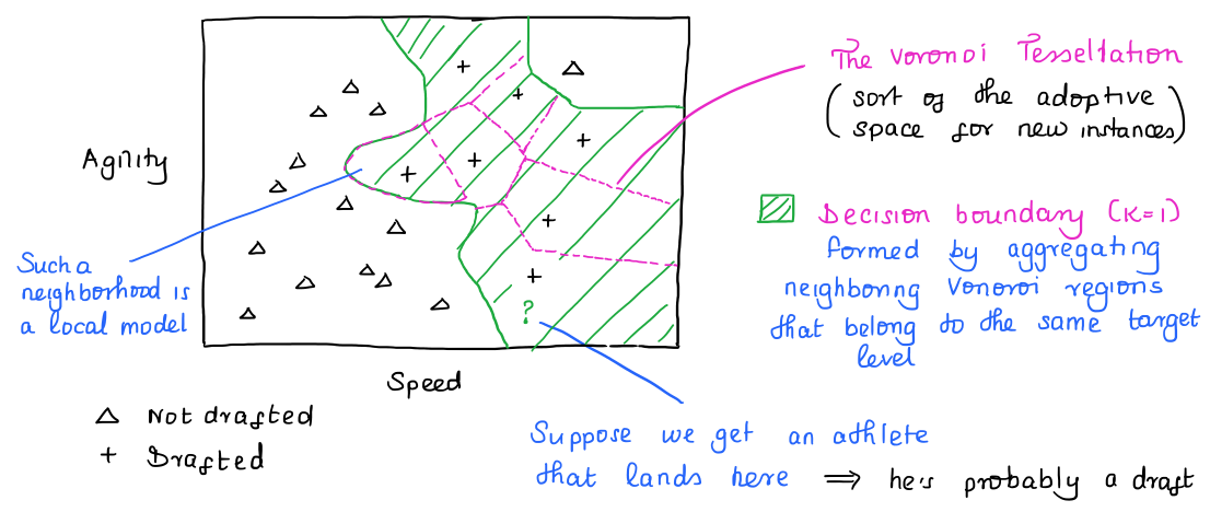
Updating the model is quite cheap. Adding an instance updates the Voronoi tessellation and therefore the decision boundary.

However, because the NN algorithm is a lazy learner (doesn’t abstract the data into a higher model), whatever savings that we make at offline time, we’ll compensate by having longer inference times.

When would anyone want to have longer inference times? It seems that reducing inference time is a crucial step for machine learning. We can do all the offline model building in fancy machines, and let even cheap machines reap the benefits of ML.

One way of making retrieval of nearest neighbors more efficient is organizing the training set into a k-d tree.